Reducing Reparameterization Gradient Variance
23 May 2017
Nick Foti, Alex D’Amour, Ryan Adams, and I just arxiv’d a paper that focuses on reducing the variance of the reparameterization gradient estimator (RGE) often used in the context of black-box variational inference. I’ll give a high level summary here, but I encourage you to check out the paper and the code.
Reparameterization Gradients
Reparameterization gradients are often used when the objective of an optimization problem is written as an expectation. A common example is black-box variational inference for approximating an intractable posterior distribution \(\propto p(z, \mathcal{D})\). The objective we typically maximize is the evidence lower bound (ELBO)
\[\begin{align} \mathcal{L}(\lambda) &= \mathbb{E}_{z \sim q(\cdot; \lambda)}\left[ \ln p(z, \mathcal{D}) - \ln q(z; \lambda) \right] \, . \end{align}\]Using gradient-based optimization requires computing the gradient with respect to \(\lambda\)
\[\begin{align} g_\lambda &= \nabla_\lambda \mathcal{L}(\lambda) \end{align}\]which itself can be expressed as an expectation. This expectation is in general analytically intractable, but we can still use gradient-based optimization if we can compute an unbiased estimate of the gradient, \(\hat g_\lambda\), such that \(\mathbb{E}[\hat g_\lambda] = g_\lambda\).
The reparameterization gradient estimator (RGE) is one such unbiased estimator. The RGE uses the “reparameterization trick” to turn a Monte Carlo ELBO estimator into a Monte Carlo ELBO gradient estimator. Recall that the reparameterization gradient estimator depends on a differentiable map, \(z(\epsilon, \lambda)\), that transforms some seed randomness, \(\epsilon \sim q_0\), such that \(z(\epsilon, \lambda)\) is distributed according to \(q_\lambda\). The RGE can be written
\[\begin{align} \nabla_\lambda \mathcal{L}(\lambda) &= \nabla_\lambda \mathbb{E}_{z \sim q(\cdot; \lambda)}\left[ \ln p(z, \mathcal{D}) - \ln q(z; \lambda) \right] \\ &= \nabla_\lambda \mathbb{E}_{\epsilon \sim q_0}\left[ \ln p(z(\epsilon, \lambda), \mathcal{D}) - \ln q(z(\epsilon, \lambda); \lambda) \right] \\ &= \mathbb{E}_{\epsilon \sim q_0} \left[ \nabla_\lambda \ln p(z(\epsilon, \lambda), \mathcal{D}) - \nabla_\lambda \ln q(z(\epsilon, \lambda); \lambda) \right] \, . \end{align}\]We can easily form an unbiased \(L\)-sample Monte Carlo estimator of \(g_\lambda\) by drawing samples \(\epsilon_1, \dots, \epsilon_L \sim q_0\) and computing
\[\begin{align} \hat g_\lambda^{(L)} &= \frac{1}{L} \sum_\ell \nabla_\lambda \ln p(z(\epsilon, \lambda), \mathcal{D}) - \nabla_\lambda \ln q(z(\epsilon, \lambda); \lambda) \end{align}\]The utility of this estimator is tied to its variance — generally, the higher the variance, the slower the optimization converges.
Method
We approach this variance reduction task by examining the generating process of the RGE, \(\hat g_\lambda\). To see what I mean, consider a single-sample estimator as a function of \(\epsilon\) (see this post for details)
\[\begin{align} \hat g_\lambda(\epsilon) &= \underbrace{ \frac{\partial \ln p(z, \mathcal{D})}{\partial z} }_{\text{data term}} \frac{\partial z(\epsilon, \lambda)}{\partial \lambda} - \underbrace{ \frac{\partial \ln q(z; \lambda)}{\partial z} }_{\text{pathwise score}} \frac{\partial z(\epsilon, \lambda)}{\partial \lambda} - \underbrace{ \frac{\partial \ln q(z; \lambda)}{\partial \lambda} }_{\text{parameter score}} \end{align}\]The gradient estimator above is a transformation of a simple random variate. It maps \(\epsilon\) — a random variable with a known distribution — to \(\hat g_\lambda(\epsilon)\) — a random variable with a complex distribution. We know this complex distribution is unbiased, but we can’t exactly compute the expectation (which is why we’re estimating it in the first place).
The key idea in this paper is that we can approximate the transformation \(\hat g_\lambda(\epsilon)\) to form a different gradient estimator. This new estimator, \(\tilde g_\lambda(\epsilon)\), is biased but has a tractable distribution. Importantly, we use the same \(\epsilon\) to form both estimators, which correlates the two random variables. We can use the biased approximation as a control variate to reduce the variance of the original RGE. This simple relationship is depicted below — the lower left is our standard reparameterization gradient; the lower right is the biased approximation.

We apply this idea to a Gaussian variational distribution \(q(z;\lambda)\). We propose a linear approximation of the transformation \(\hat g_\lambda(\epsilon)\) that results in a simple estimator, \(\tilde g_\lambda(\epsilon),\) with a known distribution (Gaussian or a shifted and scaled \(\chi^2\)).
To summarize, the unbiased Monte Carlo estimator \(\hat g_\lambda\) has a complex distribution with an uncomputable mean. The biased estimator \(\tilde g_\lambda\) has a simpler distribution with a known mean. We construct \(\tilde g_\lambda\) by approximating the process that generates \(\hat g_\lambda\). Using the same \(\epsilon\) for both estimators correlates them, making \(\tilde g_\lambda\) a powerful control variate for variance reduction.
The paper describes a way to construct a good \(\tilde g_\lambda\) that we can efficiently compute. We can do this by taking advantage of model curvature, efficient Hessian-vector products, and the stability of Gaussian random variables.
Results
We compare our gradient estimator, HVP+Local, with the pure Monte Carlo RGE. We apply these gradient estimators to two VI problems with non-conjugate posterior distributions — a hierarchical Poisson GLM and a Bayesian Neural Network — using a diagonal Gaussian variational approximation with mean parameters \(m_\lambda\) and scale parameters \(s_\lambda\) and full parameter vector \(\lambda \triangleq [m_\lambda, s_\lambda]\).
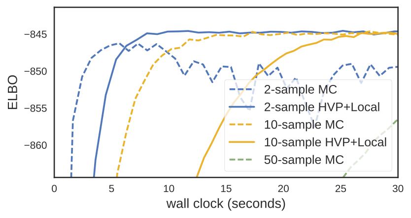
For the Poisson GLM we observe a dramatic reduction in variance for both mean and variance parameters — typically a reduction factor between 20 and 2,000x (more precise variance reduction measurements are in the paper). This reduction in variance translates to faster convergence. For the hierarchical model, we see quicker and more stable convergence:
And for the (modestly sized) Bayesian Neural Network, we see faster convergence. Note the 10-sample HVP+Local estimator outperforms the 50-sample MC estimator in terms of wall clock.
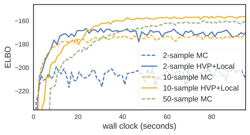
While the HVP+Local estimator requires 2–3x the computation of the pure Monte Carlo RGE, we see that this cost can be worth it. More results and details can be found in the paper.
Thanks for reading, and stay cool out there.