Natural Gradients and Stochastic Variational Inference
02 Oct 2016
Overview
My goal with this post is to build intuition about natural gradients for optimizing over spaces of probability distributions (e.g. for variational inference). I’ll examine a simple family of distributions (diagonal-covariance Gaussians) and try to see how natural gradients differ from standard gradients, and how they can make existing algorithms faster and more robust.
For concrete motivation, here’s a sneak preview of optimization improvement afforded by the natural gradient in a variational inference problem (higher values of the evidence lower bound, or ELBO, imply a better approximation)
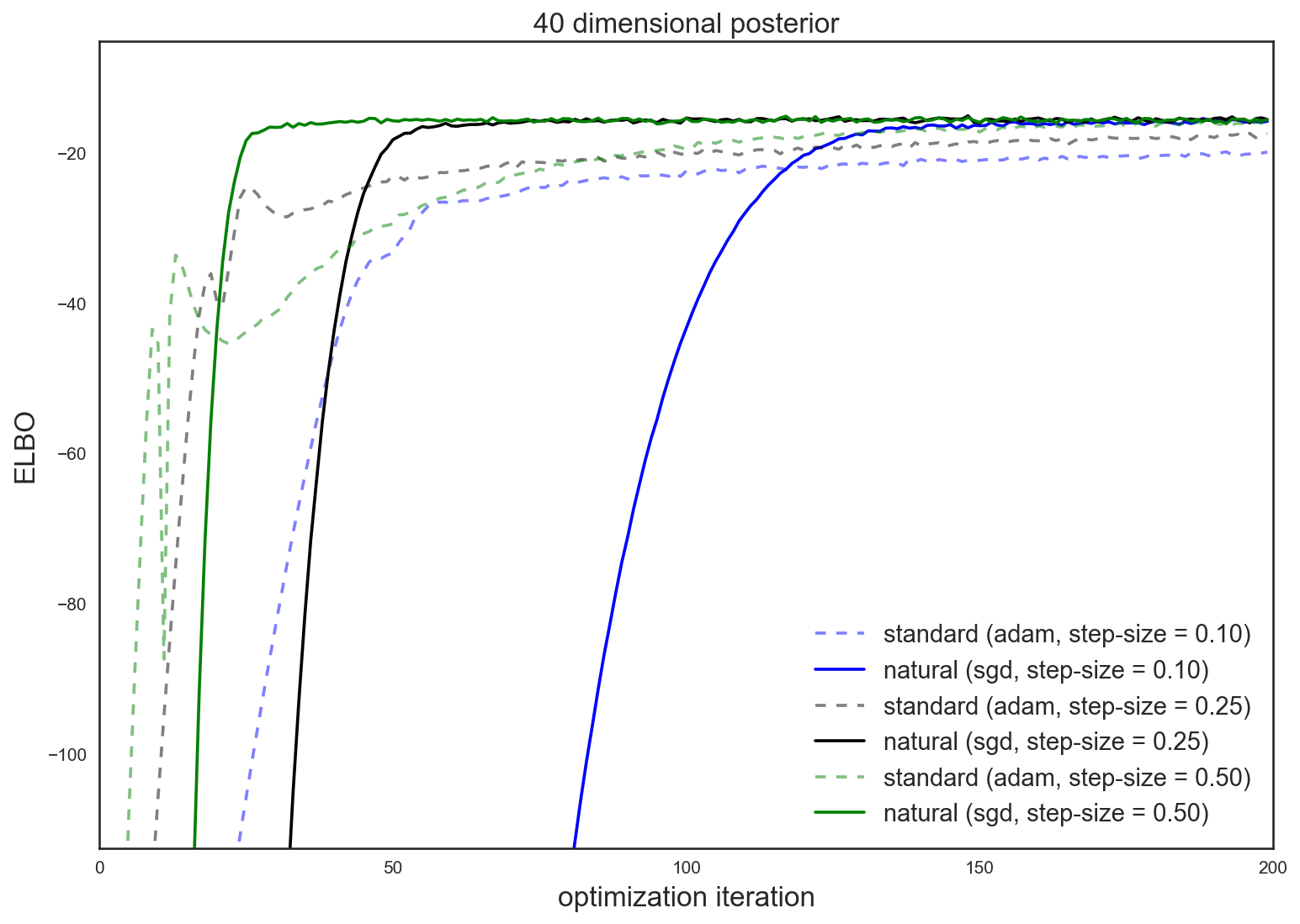
The punchline: using the natural gradient for variational inference often leads to quicker and more reliable optimization over the standard gradient. This improvement makes approximate Bayesian inference more practical for general use.
Motivation: Variational Inference
To motivate the concept of natural gradients and statistical manifolds, consider variational inference (VI), a class of methods often used for approximate Bayesian inference.
Bayesian inference typically starts with some model for data that describes a joint density, \(p(x, \mathcal{D})\), over data \(\mathcal{D}\) and model parameters (and latent variables), \(x\). This joint density is proportional to the posterior, \(p(x \,|\, \mathcal{D})\), which characterizes our beliefs about the values of parameters \(x\). Access to this distribution allows us to make Bayesian predictions, report posterior expectations, interpret posterior marginals, etc.
For notational simplicity, we drop the \(\mathcal{D}\) and denote our (unnormalized) target as \(\pi(x)\). The target is, in general, difficult to use. The VI approach is to approximate \(\pi(x)\) with some easy-to-use distribution, \(q(x; \lambda)\), parameterized by \(\lambda\) in some parameter space \(\Lambda\). VI typically proceeds by optimizing a divergence measure between \(\pi\) and \(q\) to find the \(\lambda\) that makes these distributions as similar as possible.
For VI methods, this similarity measure is typically the Kullback–Leibler (KL) divergence, \(KL(q(\cdot; \lambda) \,||\, \pi)\). The exact KL is difficult to evaluate, and for practical purposes most VI algorithms introduce an objective (known as the evidence lower bound, or ELBO) that, when maximized, corresponds to minimizing the KL. For this post, the details of the ELBO are unimportant, so we will refer to this objective simply as \(\mathcal{L}(\lambda)\) and our optimization problem is
\[\begin{align} \max_{\lambda \in \Lambda} \mathcal{L}(\lambda) \end{align}\]To sum up, solving this optimization problem is approximate Bayesian inference — a difficult integral is replaced by an easier optimization problem.
To solve this optimization problem, we’ll consider gradient-based methods, such as stochastic gradient descent (sgd), adagrad, or adam. This is where the natural gradient enters — these gradient-based methods make small moves around the parameter space, where the definition of “small” is what characterizes the difference between the natural and the standard gradient.
The next section focuses on understanding the natural gradient, and in the following section I’ll derive (and interpret) the natural gradient for a particular family of variational distributions. We’ll then see how it improves optimization in a Black-Box Stochastic VI (BB-SVI) problem for approximate Bayesian inference.
Statistical Distance
First, let’s state the obvious: each point \(\lambda \in \Lambda\) corresponds to a full probability distribution. If we ignore this, and use general-purpose gradient methods (that treat \(\Lambda\) like a Euclidean space), then we’re giving up a ton of useful structure in the problem.
To see what I mean, consider these two Gaussians, \(q_0\) and \(q_1\)
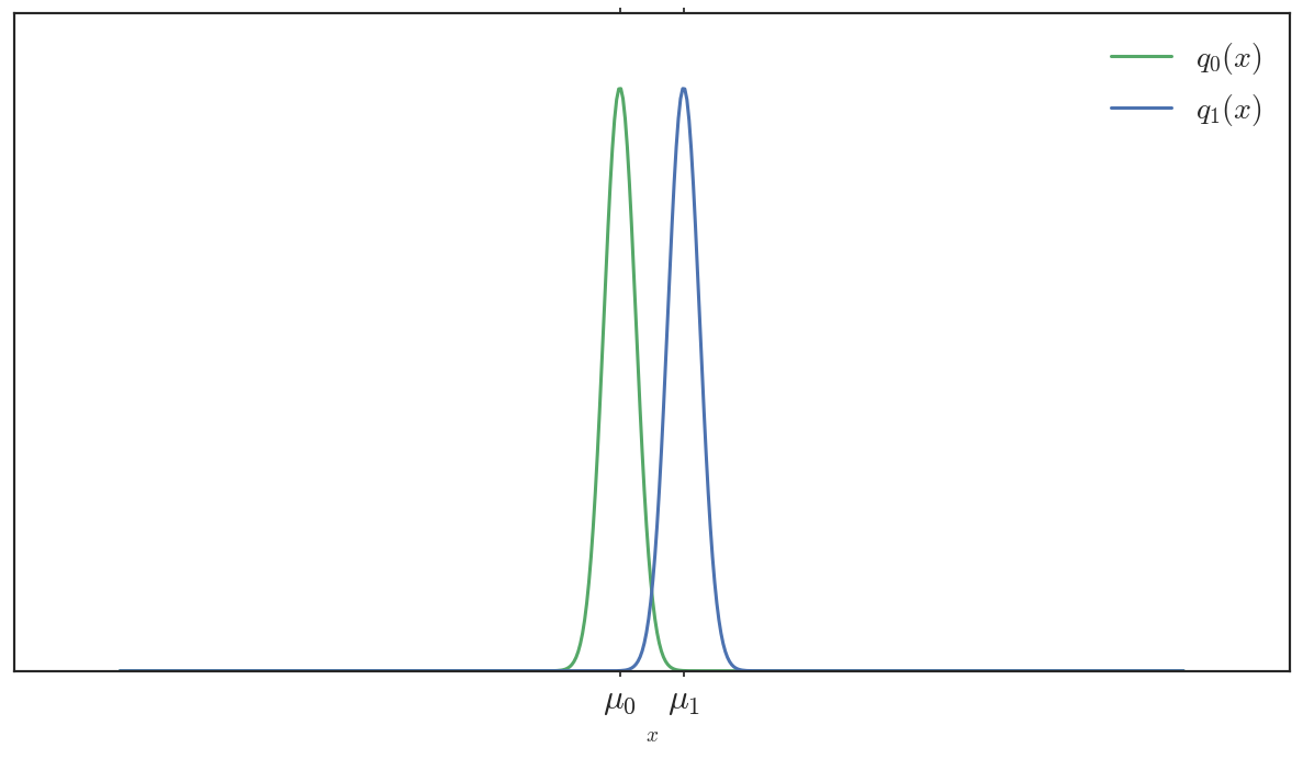
The euclidean distance between \((\mu_0, \sigma_0^2)\) and \((\mu_1, \sigma_1^2)\) is \(\sqrt{ (\mu_1 - \mu_0)^2 + (\sigma_0^2 - \sigma_1^2)^2 } = |\mu_1 - \mu_0|\) (their variances are equal, \(\sigma_0^2 = \sigma_1^2\)). However, the distributions are quite different — their support barely overlaps; samples greater than \(\mu_1\) unambiguously belong to \(q_1\) (and vice versa). More importantly, if \(q_0\) were our true target distribution, then \(q_1\) would be a poor surrogate — \(KL(q_1 || q_0)\) here is huge.
Now consider these two Gaussian distributions:
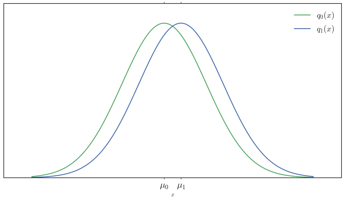
The Euclidean distance between parameters is equivalent, \(|\mu_1 - \mu_0|\). However, their support almost completely overlaps. If you saw a sample over this support, it would be difficult to distinguish which Gaussian it came from. If \(q_0\) were our true target distribution, then \(q_1\) would be a pretty good surrogate in terms of \(KL\) (not the best, but not bad).
Notably, the Euclidean distance between parameters of \(q_1\) and \(q_0\) is the same in both cases, yet the statistical distance between the top two distributions is enormous compared to the statistical distance between the bottom two. This is because naively comparing parameters ignores the structure of the objects that the parameters represent. A statistical “distance” (e.g. symmetric-\(KL\) or total variation) incorporates this information by being a functional of the entire distribution
\[\begin{align} KL(q \,||\, p) &= \int q(x) \left( \ln q(x) - \ln p(x) \right)dx = \mathbb{E}_q\left[ \ln q(x) - \ln p(x) \right] \end{align}\]When we optimize over a parameter space, we want small distances between a current value \(\lambda\) and some nearby value \(\lambda'\) to reflect this structure. The local structure defined by our choice of statistical distance defines a statistical manifold, and in order to optimize over this manifold, we need to modify our standard gradients using an appropriate local scaling, otherwise known as a Riemannian metric. This local rescaling, along with the standard gradient, can be used to construct the natural gradient.
Natural Gradient
A common Riemannian metric for statistical manifolds is the Fisher Information Matrix (“the Fisher”)
\[\begin{align} F_\lambda &= \mathbb{E}_{q(\cdot; \lambda)} \left[ \nabla_\lambda \ln q(x; \lambda) \left( \nabla_\lambda \ln q(x; \lambda) \right)^\intercal \right] \end{align}\]Another, and perhaps more intuitive way to express the Fisher Information Matrix is the second derivative of the KL divergence (which is locally symmetric)
\[\begin{align} F_\lambda &= \nabla_{\lambda'}^2 KL( \lambda' || \lambda ) \big |_{\lambda' = \lambda} \end{align}\]This blog post by Roger Grosse goes into more detail on the Fisher Information Matrix, and how it pops up as the Riemannian Metric for statistical manifolds.
For gradient-based optimization methods, we can replace standard gradients with the natural gradient
\[\begin{align} \tilde \nabla_\lambda &= F_\lambda^{-1} \nabla_\lambda \mathcal{L}(\lambda) \end{align}\]which corresponds to the direction of steepest ascent along the statistical manifold. This blog post (by Nick Foti) does a great job describing the natural gradient, and why it corresponds to this direction.
To better understand the natural gradient, let’s take a closer look at the Fisher for a simple class of distributions: diagonal Gaussians.
Gaussian Example
Perhaps the simplest (and most common) approximate posterior distribution is a diagonal Gaussian. Consider diagonal Gaussian distributions parameterized by \(\lambda = [\mu_1, \dots, \mu_D, \ln \sigma_1, \dots, \ln \sigma_D]\), where \(\mu\) is the mean vector and \(\sigma_1, \dots, \sigma_D\) are the standard deviations (i.e. the square root of the diagonal of the covariance matrix). For convenience, we refer to means as \(\mu_d\) and the log standard deviations as \(\lambda^{(sd)}_{d}\) In this instance, the natural gradient is easy to derive and cheap to compute.
To derive the Fisher, we first look at the gradient of the log density of a diagonal Gaussian (note that \(\ln |\Sigma|\) for a diagonal matrix is \(\sum \ln\sigma^2_{dd} = \sum 2 \ln \sigma_{dd}\))
\[\begin{align} \ln q(x; \lambda) &= -\frac{D}{2}\ln 2\pi - \frac{1}{2} \sum_d 2\lambda^{(sd)}_d -\frac{1}{2} \sum_{d} \exp(-2\lambda^{(sd)}_d)( x_d - \mu_d)^2 \\ \frac{\partial \ln q}{\partial \mu_d} &= (x_d - \mu_d) \exp(-2 \lambda^{(sd)}_d) = \frac{(x_d - \mu_d)}{ \sigma_d^2 } \\ \frac{\partial \ln q}{\partial \lambda^{(sd)}_d} &=(x_d - \mu_d)^2 \exp(-2\lambda_d^{(sd)}) - 1 = \frac{(x_d - \mu_d)^2}{\sigma_d^2} - 1 \\ \end{align}\]The Fisher information matrix is the outer product of this gradient.
To obtain an analytical form for the Fisher, consider its first \(D\) diagonal terms, corresponding to components of the mean vector, \(\mu_d\)
\[\begin{align} (F_\lambda)_{d,d} &= \frac{\mathbb{E}\left[ (x_d - \mu_d)^2 \right]}{(\sigma_d^2)^2} = \frac{\sigma_d^2}{(\sigma_d^2)^2} = \frac{1}{\sigma_d^2} \end{align}\]The off diagonal term corresponding to components \(\mu_d\) and \(\mu_d'\) is easily seen to be zero (due to independence of dimensions)
\[\begin{align} (F_\lambda)_{d,d'} &= \mathbb{E}\left[ (x_d - \mu_d)(x_{d'} - \mu_{d'})\right] / \sigma_d^2 \sigma_{d'}^2 = \texttt{Cov}(x_d, x_d') / \sigma_d^2 \sigma_{d'}^2 = 0 \end{align}\]The off diagonal term corresponding to \(\mu_d\) and \(\lambda^{(sd)}_{d'}\) is also 0
\[\begin{align} (F_\lambda)_{d,2d'} &= \mathbb{E} \frac{(x_d - \mu_d)}{ \sigma_d^2 } \left( \frac{(x_{d'} - \mu_{d'})^2}{\sigma_{d'}^2} -1 \right) \\ &= \frac{\mathbb{E}(x_d - \mu_d)}{ \sigma_d^2 } \frac{\mathbb{E}(x_{d'} - \mu_{d'})^2}{\sigma_{d'}^2} \\ &= 0 \end{align}\]Lastly, the diagonal term for \(\lambda^{(sd)}_d\) is
\[\begin{align} (F_\lambda)_{2d,2d} &= \mathbb{E} \left(\frac{(x_d - \mu_d)^2}{\sigma_d^2} - 1\right)^2 \\ &= \mathbb{E} \left(\frac{(x_d - \mu_d)^2}{\sigma_d^2}\right)^2 - 2 \frac{(x_d - \mu_d)^2}{\sigma_d^2} + 1 \\ &= \frac{1}{\sigma_d^4} \mathbb{E} (x_d - \mu_d)^4 - \frac{2}{\sigma_d^2} \sigma_d^2 + 1 \\ &= \frac{3 \sigma^4}{\sigma_d^4} - 1 = 2 \end{align}\]which makes use of the fact that the fourth central moment of a normal is known to be \(3\sigma^4\).
In summary, the Fisher for a diagonal Gaussian parameterized by \(\lambda = [\mu_1, \dots, \mu_D, \ln \sigma_1, \dots, \ln \sigma_D]\) is simply
\[\begin{align} F_\lambda &= \texttt{diag}\left( \frac{1}{\sigma_1^2}, \dots, \frac{1}{\sigma_D^2}, 2, \dots, 2 \right) \end{align}\]Examining the Fisher for diagonal Gaussians allows us to see exactly how the natural gradient differs from the standard gradient. If a dimension \(d\) has small variance, then preconditioning by the inverse Fisher makes the natural gradient smaller along the mean dimension, \(\mu_d\). Intuitively, this makes sense — we want our optimization routine to slow down when the component variance is small because small changes to the mean correspond to big changes in KL (see the two skinny Gaussians above), which can result in chaotic looking optimization traces. When the variance along a dimension is large, the inverse Fisher elongates the standard gradient along that dimension. Again, this makes sense — when the component variance is high we can move the mean a lot farther (in Euclidean distance) without moving that far in terms of KL (see the two wide Gaussians above). This means that natural gradient SGD moves a lot faster along this dimension when we’re in a region of space that corresponds to higher \(q\) variance. This automatic scaling is a benefit of incorporating local metric information in our optimization procedure.
The added bonus is that the Fisher, in this case, is essentially free to compute.
BB-SVI Example
I wrote a simple autograd example
(built on the existing BB-SVI example)
to illustrate how the behavior
of the natural gradient differs from the standard gradient.
In this case, the posterior is a multivariate normal model with a
non-conjugate prior.
Optimizing the variational objective results in the following ELBO traces (higher implies a better approximation)
For all step-sizes I tried, using momentum-less sgd and the natural gradient found
a better solution (or converged much more quickly) than using adam with the
standard gradient. In most instances, adam makes quick progress
early on (potentially accompanied by some instability), but sgd + natural
gradient catches up and converges more quickly.
These results are even more pronounced in a higher dimensional \(D = 400\) experiment
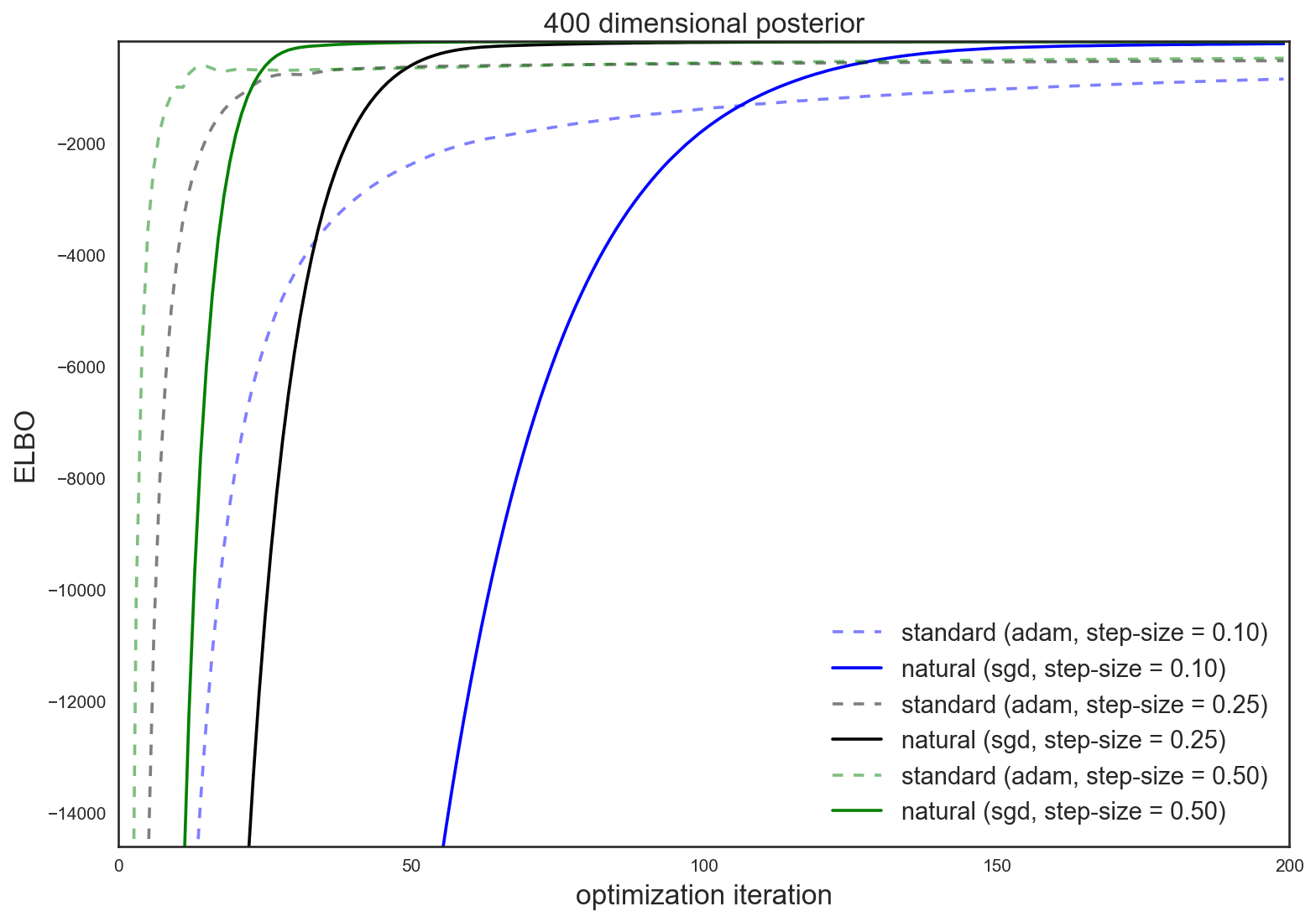
The natural gradient is intuitive, easy and cheap to use, and often attains superior and quicker results than the standard gradient.
And that’s something we can all cheer about.
(Thanks Matt Johnson for sanity checking this post and helping me understand most of these concepts!)
Edit: Antti Honkela pointed me to work he and colleagues published back in 2010: Approximate Riemannian Conjugate Gradient Learning for Fixed-Form Variational Bayes. In it, they use natural gradients of variational parameters and conjugate gradients (along with comparison to gradient descent methods) to optimize the variational objective, and show more reliable results over standard gradients. Check out the paper and references therein for more details.