Andrew Miller

Expectation Maximization and Gradient Updates

15 Oct 2015

There are many ways to obtain maximum likelihood estimates for statistical models, and it’s not always clear which algorithm to choose (or why). There appears to be a natural divide between fixed-point iterative methods, such as Expectation Maximization (EM), and directly optimizing the marginal likelihood with gradient-based methods. One great reference that bridges this gap is the paper Optimization with EM and Expectation-Conjugate-Gradient by Salakhutdinov, Roweis and Ghahramani from ICML in 2003. The main takeaway of the paper is that an EM iteration can be viewed as a preconditioned gradient step on the marginal likelihood.

The model setup includes observed data, \(x\), latent variables, \(z\), and model parameters \(\Theta\). To fit the model, our goal is to maximize the marginal likelihood of the observed data:

\[L(\theta) \equiv \log p(x | \Theta) = \log \int p(x, z | \Theta) dz\]

####Expectation-Maximization The standard EM algorithm is often presented in a terse, unintuitive way:

• E-Step: compute \(Q(\Theta | \Theta^{(t)}) = E_{p(z | x, \Theta^{(t)})} [ \log p(x, z | \Theta) ]\)
• M-Step: compute \(\Theta^{(t+1)} = \arg\max_\Theta Q(\Theta | \Theta^{(t)})\)

We can unpack the two steps by examining the marginal likelihood itself.

\[\begin{align} L(\Theta) &= \log p(x | \Theta) = \log \int p(x, z | \Theta) dz \\ &= \log \int \frac{p(z | x, \Psi)}{p(z|x, \Psi)} p(x, z | \Theta)dz \\ &= \log E_{\Psi}\left( \frac{ p(x, z| \Theta)}{p(z | x, \Psi)} \right) \\ &\geq E_{\Psi} \left( \log p(x, z | \Theta) - \log p(z | x, \Psi) \right) &\text{ Jensen's } \\ &= \underbrace{E_{\Psi} \log p(x, z | \Theta)}_{\text{ECDLL}} \underbrace{-E_{\Psi}\log p(z | x, \Psi)}_{\text{Entropy}} \\ &= Q(\Theta, \Psi) + H(\Psi) \equiv F(\Theta, \Psi) \end{align}\]

where we have introduced auxiliary parameters \(\Psi\). The EM algorithm the proceeds

• E-step: maximize \(F\) with respect to \(\Psi\) holding \(\Theta\) fixed [¹]
• M-step: maximize \(F\) with respect to \(\Theta\) holding \(\Psi\) fixed

So EM is optimizing a (sometimes tight) lower bound on the log marginal likelihood by alternately maximizing \(\Psi\) and \(\Theta\). We can think of one EM update as a mapping \(M\), that is \(\Theta^{(t+1)} = M(\Theta^{(t)})\), and examine the properties of this mapping in terms of the pieces of the functional \(F\). First, we note that if EM is at a stable point, \(\Theta^*\), such that \(\Theta^* = M(\Theta^*)\), then around \(\Theta^*\) by a Taylor series expansion, the mapping can be approximated

\[\begin{align} M(\Theta) &\approx \Theta^* + M'(\Theta^*)(\Theta - \Theta^*) \\ \implies \Theta^{(t+1)} - \Theta* &\approx M'(\Theta^*)(\Theta^{(t)} - \Theta^*) \end{align}\]

and convergence near the optimum relies on the structure of the Jacobian matrix of the EM mapping.

####EM as a gradient update

Now the question is, how can we relate the EM step, \(\Theta^{(t)} \mapsto \Theta^{(t+1)}\), to the gradient of the marginal likelihood, \(\nabla L(\Theta)\)? The authors of the paper claim that an EM step can be written

\[\begin{align} \Theta^{(t+1)} - \Theta^{(t)} &= P(\Theta^{(t)}) \nabla L(\Theta) \end{align}\]

and provide conditions where \(P(\Theta^{(t)})\) exists (C1 and C2 in the paper). In order to gain some insight about the form of \(P(\Theta^{(t)})\), we can differentiate above with respect to \(\Theta^{(t)}\)

\[\begin{align} M'(\Theta^{(t)}) - I &= P'(\Theta^{(t)}) \nabla L(\Theta^{(t)}) + P(\Theta^{(t)}) S(\Theta^{(t)}) \end{align}\]

where

\[\begin{align} S(\Theta^{(t)}) &= \frac{ \partial L(\Theta) }{\partial \Theta^2} \big\vert_{\Theta^{(t)}} \\ M'(\Theta^{(t)}) &= \frac{\partial \Theta^{(t+1)}}{\partial \Theta^{(t)}}\big\vert_{\Theta^{(t)}} \end{align}\]

and the authors argue that when the optimizer is in a flat region of \(L\) (small \(\nabla L\) and \(P'(\Theta^{(t)})\) is not too big), the rightmost term will dominate. So roughly

\[\begin{align} P(\Theta^{(t)}) &\approx -\left( I - M'(\Theta^{(t)}) \right) S(\Theta^{(t)})^{-1} \end{align}\]

Examining the above equation, convergence is generally controlled by the eigenvalues of \(M'(\Theta^{(t)})\). If the eigenvalues of \(M'(\Theta^{(t)})\) are small, then the EM update looks like a Newton update

\[\begin{align} \Theta^{(t+1)} \approx \Theta^{(t)} - S(\Theta^{(t)})^{-1} \nabla L(\Theta^{(t)}) \end{align}\]

but if the eigenvalues of \(M'(\Theta^{(t)})\) are large, then the step-size ends up being very small, leading to slow convergence.

We can gain some insight into the spectral structure of the EM iteration by looking at the result from the original EM paper [²] paper that discusses the gradient of the EM map. If EM converges to some point \(\Theta^*\), then

\[\begin{align} \frac{\partial M(\Theta)}{\partial \Theta} \big\vert_{\Theta = \Theta^{*}} &= \underbrace{\left[ \frac{\partial^2 H(\Theta, \Theta^*)}{\partial \Theta^2} \big\vert_{\Theta=\Theta^*} \right]}_{\text{posterior info}} \underbrace{\left[ \frac{\partial^2 Q(\Theta, \Theta^*)}{\partial \Theta^2} \big\vert_{\Theta=\Theta^*}\right]^{-1}}_{\text{complete data info}} \end{align}\]

which describes the “ratio of missing information” near the optimal value \(\Theta^{*}\) - the derivative of the EM map is equal to the ratio of posterior information and the complete data information (w.r.t. the latent variable posterior expectation). The authors combine the above into the relationship to claim that near the point of convergence

\[\begin{align} P(\Theta^{(t)}) \approx \left[ I - \left( \frac{\partial^2 H}{\partial \Theta^2}\right) \left( \frac{\partial^2 Q}{\partial \Theta^2}\right)^{-1} \big\vert_{\Theta=\Theta^{(t)}} \right] \left[ -S(\Theta^{(t)})\right]^{-1} \end{align}\]

which makes it clear that when the ratio of “missing information” to “complete information” is low, EM updates look more like Newton updates that make use of the curvature of the log marginal likelihood. However, when “missing information” is a large fraction of the “complete information”, EM updates take small steps that lead to slow convergence.

A simple simulation for a 2-component mixture of Gaussians illustrates this point. I ran EM on two different mixtures of Gaussians a well separated and a not-so-well separated model:

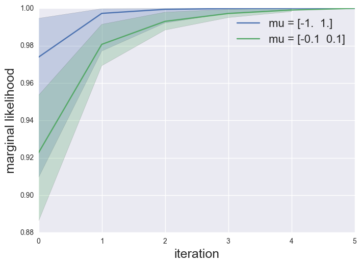
the median convergence for the not-so-well separated model (less “information”) is on average slower (though EM is very quick to converge in both examples). The paper provides empirical evidence that linear dynamical systems and HMMs tend to really show slow EM convergence (compared to gradient updates).

####Proposed Method: Hybrid EM-CG updates This intuition gives us a simple rule: if we observe that posterior uncertainty is high in a particular region of our parameter space, we shouldn’t do an EM update and instead do a gradient-based step. If we observe posterior uncertainty is low, then we can incorporate computationally inexpensive hessian information by doing an EM update.

The author’s propose using the (normalized) posterior entropy at each step as a heuristic for deciding when to switch between conjugate gradient updates and EM updates (this seems to just be for discrete models). It works well - it seems to almost always improve upon EM (which often slows to a crawl near the point of convergence), and will sometimes improve upon CG only updates (in general it doesn’t seem to do worse).

######Questions? The authors established an approximate relationship between standard gradient-based updates and EM iterations, and what we learned boils down to is: the more (relative) information about \(z\) that is available, the more curvature information EM allows us to use for an update. But when \(z\) doesn’t contain a lot of information, then taking expectations with respect to it won’t get us much traction, and updates will be slow.

But heuristically switching between two different types of optimization methods seems unsatisfying. Can an optimization routine enjoy the curvature information that EM (will sometimes) provide while more continuously relying on on pure gradient-based updates? Perhaps one can specify a “coarsened” latent variable model that admits the same marginal likelihood, but for which our current data is highly informative, and iterate in that space.

Also, due to close relationship between EM iterations and Gibbs updates, what can we learn about MCMC routines from this paper? When does it make sense to perform a Gibbs update (or more realistically, a “something”-within-Gibbs \(z \vert \Theta\)) and when does it make sense to just perform a marginal MCMC update for \(\Theta\)?

---