Improving Variational Approximations
23 Nov 2016
Nick Foti, Ryan Adams, and I just put a paper on the arxiv about improving variational approximations (short version accepted early to AABI2016). We focused on one problematic aspect of variational inference in practice — that once the optimization problem is solved, the approximation is set and there isn’t a straightforward way to improve it, even when we can afford some extra compute time.
Markov chain Monte Carlo methods have a simple solution — run the chain for more steps and the posterior approximation will get better and better. Variational inference (VI) methods, on the other hand, typically pre-specify some class of approximating distributions, and then optimize the VI objective. When that pre-specified class of distributions (the variational family) doesn’t include the neighborhood around the target distribution, the resulting VI solution will still be sub-optimal, in that there will be a non-zero KL-divergence between the approximation and the target. This will result in biased posterior estimates.
There is a ton of great work toward solving this problem (more examples cited in the paper), including:
- Dustin Tran and Rajesh Ranganath have put out an awesome series of papers that allow for more expressive distributions, based on marginalizing out a latent variable, to be used as variational approximations [1], [2].
- Danilo Rezende and Shakir Mohamed introduced the normalizing flows framework [3], which constructs an expressive approximate distribution by composing invertible maps.
In the above approaches, the variational family is made to be expressive from the start, and the evidence lower bound (ELBO), or a surrogate, is optimized as usual.
In our approach, we first specify a simple class of approximations — e.g. Gaussians with diagonal covariance — and then optimize the corresponding variational objective, resulting in the best reachable approximation (in the KL-sense) that a diagonal Gaussian can do. We then expand the variational family in one of two ways:
- add structure to the covariance
- add a component and form a mixture
With the new degrees of freedom afforded by the additional covariance or mixture component parameters, we can define a new variational objective and optimize.
Low rank + diagonal covariance structure
Mean field variational inference (MFVI) proposes a fully factorized approximate distribution, which trades expressiveness for computational/algorithmic tractability. This can lead to poor approximations, particularly when the true posterior has some highly correlated dimensions.
On the other end of the spectrum, using a full, \(D\times D\) covariance matrix might be overkill, as some dimensions of the posterior may be (approximately) independent. Furthermore, as the necessary operations are typically \(O(D^3)\), a full covariance matrix may be computationally prohibitive in high dimensions.
To strike a balance, we propose rank \(r\) plus diagonal covariance structure
\[\begin{align} \Sigma &= CC^\intercal + \text{diag}(\sigma_1^2, \dots, \sigma_D^2) \end{align}\]where \(C \in \mathbb{R}^{C \times r}\), which allows necessary covariance manipulations to be done in \(O(r^3 + D)\) time.
As an example, here is a representative sample of four bivariate marginals from a D = 37-dimensional posterior (resulting from a hierarchical Poisson GLM) — note that there are a devilish 666 total pairwise covariances to model in this real-data posterior. With a diagonal covariance (D covariance parameters) we see the typical under-estimation of marginal posterior variance
![]()
(in all images, samples and histograms result from running MCMC for 20k samples)
Additional low rank structure introduces the capacity to capture additional correlations. Rank one covariance (2D covariance parameters):
![]()
Rank two covariance (3D covariance parameters):
![]()
Each new rank can “find” a direction in parameter space that corresponds to a posterior correlation. Accurately accounting for posterior correlation allows the approximation to obtain more accurate marginal variance estimates. Below is a comparison of MFVI (diagonal covariance) and MCMC (NUTS) on six univariate marginals from the same 37-dimensional posterior.
![]()
And below are the rank-three covariance univariate marginals.
![]()
The marginal variances now much better reflect the true posterior’s uncertainty — and at a much cheaper cost than the \(D\times D\) full rank parameterization. It is quick and easy to fit this low rank + diagonal variational family to a very general class of posteriors using black-box VI — details in the paper!
Adding mixture components
Once we’ve settled on a covariance rank, we can further improve the approximation by adding components to form a mixture. This creates a new variational objective — an objective that is a function of the new mixing weight and the new component parameters. In our paper, we show how to fit these parameters with stochastic gradients obtained via the “re-parameterization trick” [4].
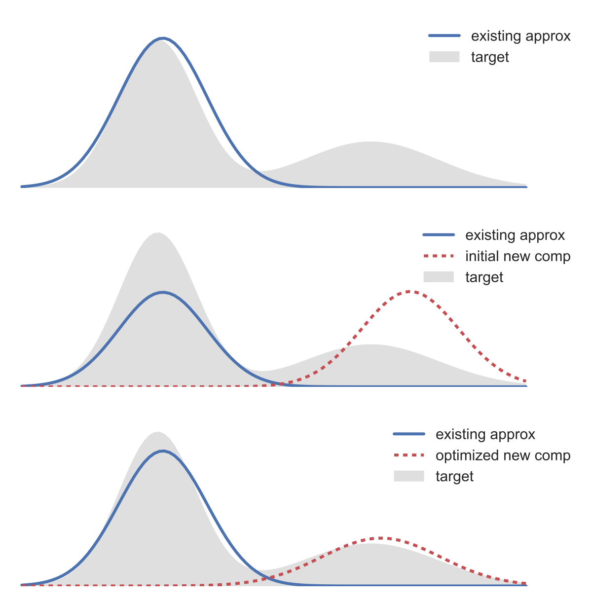
The idea (illustrated below) is quite simple — (i) fit an existing approximation; (ii) initialize a new component; (iii) optimize the ELBO as a function of the new component parameters.
This allows us to capture non-Gaussianity in the posterior. Below is another real-data example; we plot a bivariate marginal from a 20-dimensional hierarchical model.

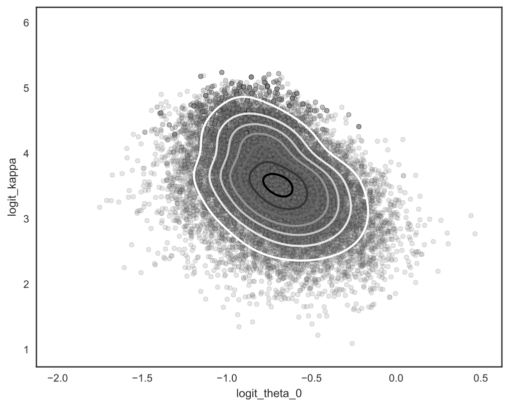
We found that this variational boosting procedure can be quite sensitive to new component parameter initialization — our paper discusses an intialization technique that empirically assuages some of this sensitivity. This is definitely an active area of research.
We also like to mention independent and concurrent work from Fangjian Guo et al. that was recently submitted to the arxiv; the authors describe a similar procedure for incorporating new mixture components into a variational approximation. They show that this greedy procedure will reduce the KL objective (as a function of the new mixing weight); and they detail a method for fitting new component parameters. Our work focuses more on adapting the reparameterization trick for mixture distributions, and incorporating covariance structure to reduce the number of mixture components required to describe posterior correlation. It’s really interesting and complimentary to our work, and I encourage you to check it out!
And on that note, Happy Thanksgiving!

[1] Ranganath, Rajesh, Dustin Tran, and David M. Blei. “Hierarchical Variational Models.” arXiv preprint arXiv:1511.02386 (2015).
[2] Tran, Dustin, Rajesh Ranganath, and David M. Blei. “Variational Gaussian Process.” arXiv preprint arXiv:1511.06499 (2015).
[3] Rezende, Danilo Jimenez, and Shakir Mohamed. “Variational inference with normalizing flows.” arXiv preprint arXiv:1505.05770 (2015).
[4] Kingma, Diederik P., and Max Welling. “Auto-encoding variational bayes.” arXiv preprint arXiv:1312.6114 (2013).